Spatio-Temporal Soil Mapping: Linkage Between Soil Types and Property Units
Posted on May 1, 2024 • 8 min read • 1,562 wordsVisualising Correlation between Soil Types and Property Units Using OSM data

Investigating Soil Patterns: FME - PostGIS - ArcGIS Approach
The aim of this assignment is to provide an insight in how soil types could affect the living conditions for individuals in the parish Hög in Sweden and to prepare a harmonized database that can be used as a tool for such an analysis. Specifically, the task is to find a linkage between soil types and property units in Hög. With that information it is possible to derive information about how the individual farmers may have cultivated their land and how the dominating soil types changed throughout the years.
Data
Historical data for the property units in Hög was provided for this study, showing the geographical extent of each property unit and their change with time. The time period ranges from the year 1800 to 1900 (Hog_LSM_EM). Also used was a soil dataset for the area created by the Swedish Geological Survey (SGU). It contains modern soil data for Hög and nearby parishes (Jordart_25_100k_jg2). For background information OpenStreetMap (OSM) feature layers were obtained, source: http://www.openstreetmap.org/. They consist of eight layers showing different feature types covering the entire Sweden. The OSM layers are in the reference system WGS84. Further properties of the soil and property units datasets are listed here below, as well as maps that showcase what they look like.
Table 1. Properties of Hog_LSM_EM(property) table.
| Hog_LSM_EM | ||
|---|---|---|
| Columns | Data Type | Description |
| objectid | integer | Unique identifier |
| parish | string | Name of parish |
| code | string | Code of property unit |
| codepart | string | Some property units have a letter after the code in the property unit name |
| name | string | Name of parish |
| mapseries | string | Name of map series |
| property_u | string | Name of property unit |
| obsdate | string | Observation date of the property |
| startdate | string | Start date of the property |
| enddate | string | End date of the property |
| objectid_1 | integer | Unique identifier |
| geom | geometry | Polygon data |
| Data Format : ESRI Shape | ||
| Coordinate System: SWEREF99TM EPSG: 3006 |
Table 2. Properties of Jordart_25_100k_jg2(soil) table.
| jordart_25_100k_jg2 | ||
|---|---|---|
| Columns | Data Type | Description |
| jg2 | integer | soil code |
| jg2_tx | string | text description for soil type |
| kartering | string | are classification |
| karttyp | integer64 | type of map |
| symbol | integer | code for symbolization |
| shape_area | double | area of polygon |
| shape_length | double | perimeter of polygon |
| eng_soil | string | English name of soil type |
| objectid | integer | Unique identifier |
| geom | geometry | Polygon data |
| Data Format : ESRI Shape | ||
| Coordinate System: SWEREF99TM EPSG: 3006 |
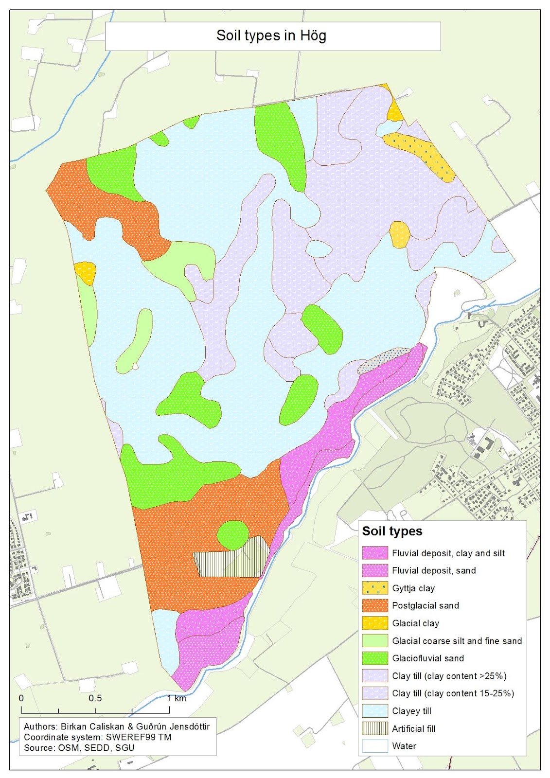
Figure 1. Soil types in Hog
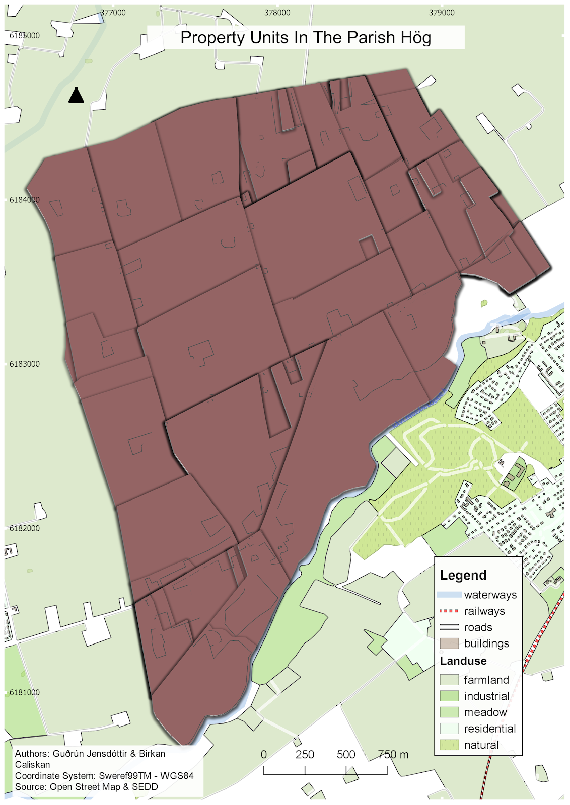
Figure 2. A view of property unit objects while the OSM features are used as a base map.
Methodology
The methodology for the study can be described in three parts. First, preprocessing and preparation of the data was done using FME. From there it was sent to a PostGIS server where approriate spatial queries were made for the analysis. And lastly visualisations and further analysis of the features created in PostGIS were performed both in QGIS and ArcMap.
FME
In order for OSM objects to be used for illustration purposes, this dataset should be preprocessed prior to PostGIS transfer. Thus, the objects of OSM dataset were reprojected into SWEREF99TM and clipped according to the boundaries of a box made with the CREATOR tool. This boundary box was created by considering a 4 km buffer zone from the extent of the dissolved property units. The output objects were sent to the server using a PostGIS writer for the following analysis. The flowchart showing the steps taken here can be seen in appendix A.
The provided shapefiles “jordart_25_100k_jg2”(soil) and “HOG_LSM_EM”(property) are already projected into SWEREF99TM(EPSG:3006), therefore both data were saved in a file geodatabase and subsequently were send our PostGIS server. Prior to the transfer, the English name of the soil types was joined in the FME environment from an excel table which included names in both Swedish and English. The join was done by using “AttributeValueMapper”. Unwanted fields such as Karttype, Shape_length were removed as these records are not relevant to our analysis. Because of the fact that the soil dataset covers a larger area than the boundary of Hög, it need to be clipped according to the parish outer borders.
Therefore, the polygons of property file were dissolved into one geometry to represents the boundary of Hög and then this geometry was used as a clipper input for the CLIPPER function, while the soil types were defined as the clippee.
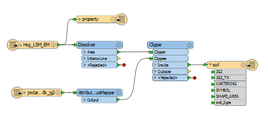
Figure 4. A screenshot from FME software representing the operations performed for Soil and property objects.
PostGIS
In order to calculate the most dominating soil types, the soil and property features should be intersected. In the PostGIS environment, The command “ST_Intersection” returns geometric intersections of the input features(soil.geom, property.geom). The output geometries are saved under the geom column. Since we want to rank the most three dominating soil types for each property unit, the areas of “geom” were calculated and saved to the area column. This is the query used for the intersection:
CREATE TABLE intersected AS

SELECT

property.objectid, soil.soil_type,obsdate, startdatem, enddatem, ST_AREA(ST_INTERSECTION(soil.geom, property.geom)) AS area, ST_INTERSECTION(soil.geom, property.geom) AS geom

FROM

soil, property

WHERE

ST_AREA(ST_INTERSECTION(soil.geom, property.geom)) > 0

GROUP BY

soil.geom, property.geom, property.objectid, soil.soil_type,obsdate, startdatem, enddatem

ORDER BY

property.objectid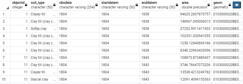
Figure 4. First 10 records from the intersected table
To minimize redundancy of the data, the soils that are of the same type within each property unit at a specific time were merged in one and the sum of their areas calculated. By using ST_Union coupled with GROUP BY the merging was performed on the geometry of the intersected layer and SUM was performed on the area column. The query that was used (see next page) returns a new table which includes distinct soil types per each property unit.
CREATE TABLE soil_per_unit AS

SELECT

objectid, soil_type, obsdate, startdatem, enddatem,SUM(area) as area, ST_Union(geom) as geom

FROM intersected

GROUP BY

soil_type, objectid, obsdate, startdatem, enddatem

ORDER BY

objectid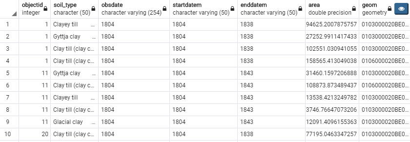
Figure 5. First 10 records from soil_per_unit table
The next query (see below) was made to rank three dominating soil types for each property unit and to calculate the percentage of soils. It creates a new column containing rank values, which are calculated based on the magnitude of the values in the area column. Partition by was defined to “objectid” as we need to rank the total area of polygons by grouping the same object values. The areas of polygons are listed in descending order and the results are limited to only the first three soil types by “where area_rank <=3” definition.
CREATE TABLE percentage as

SELECT

*, (area*100/SUM(area) OVER(PARTITION BY objectid)) as percentage from

(

SELECT

*, rank() over(partition by objectid order by area desc) area_rank

FROM

soil_per_unit

) AS rank

WHERE

area_rank <=3
The following block of code “(area*100/SUM(area) OVER(PARTITION BY objectid)) as percentage” groups each property unit by defining objectid as a parameter in PARTITION BY and divides each polygon area to sum of the total area of the objectid. Thereby, the three dominating soils in each property unit and their percentages are computed and saved in the new table, called “percentage”.
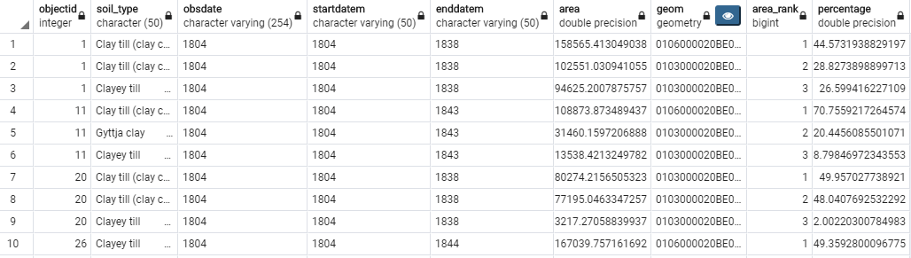
Figure 6. First 10 records from percentage table.
QGIS and ArcMap
To visualise the data both QGIS and ArcMap were used. To use it in ArcMap, the data were exported as shapefile from the QGIS environment. From there a “time slider” was utilized to create a animation of the different soil types dominating each property unit throughout the period 1804-1904
Results
Resulting from the analysis were several output data that are stored in the PostGIS environment, specifically the intersected features of soil and property units and a layer that shows the area and percentage of the three dominating soil types per unit.
Table 3. Properties of the end table created in PostGIS environment
| percentage | ||
|---|---|---|
| Column name | Data Type | Description |
| objectid | integer | Unique identifier |
| soil_type | char(50) | Soil type |
| obsdate | string | Observation date of the property |
| startdate | string | Start date of the property |
| enddate | string | End date of the property |
| geom | geometry | Polygon data |
| area | double precision | Area of soils (m2) |
| percentage | double precision | percentage of soil type per individual |

Figure 7. A view that represents the objects from the “percentage” table in pgAdmin4 environment.
The animation below represents the most dominating soil type for each property unit and how soil types change through the years 1804 to 1912. The color palette of this animation is as specified in the file Jordart, grundlager.lyr, which accompanied the soil data.
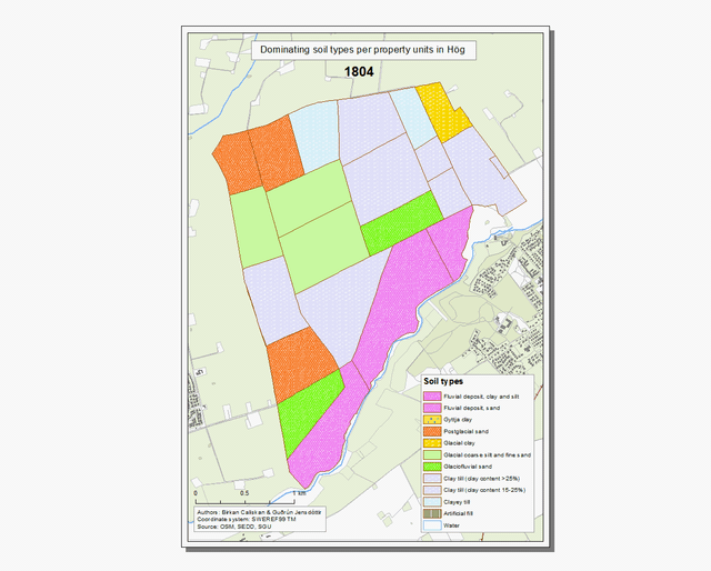
Figure 8. The animation for the alteration of the most dominating soil type in each property unit through time.
The database that was created can be used in further demographic research in the study of living conditions of individuals. On it’s own it is reflective of how farmers may have cultivated their land throughout time and provides a useful insight in how individuals lived in different time periods. Some property units go through stark changes in size and shape, resulting in different dominating soil types for each period, while others remain more or less the same. As an example, the soil changes in property unit Hög 11 can be seen below.
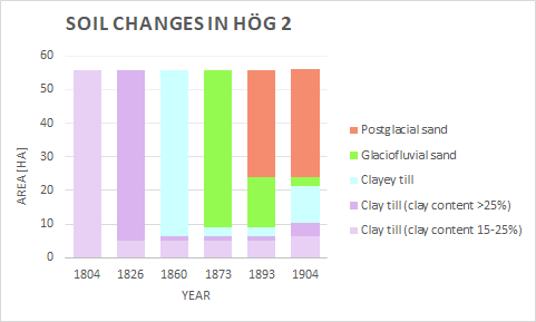
Fig 9. Changes in dominating soil types for property unit “Hög 2”. This is the second largest property unit in the parish and demonstrates the changes that may take place in soil types throughout the time range.
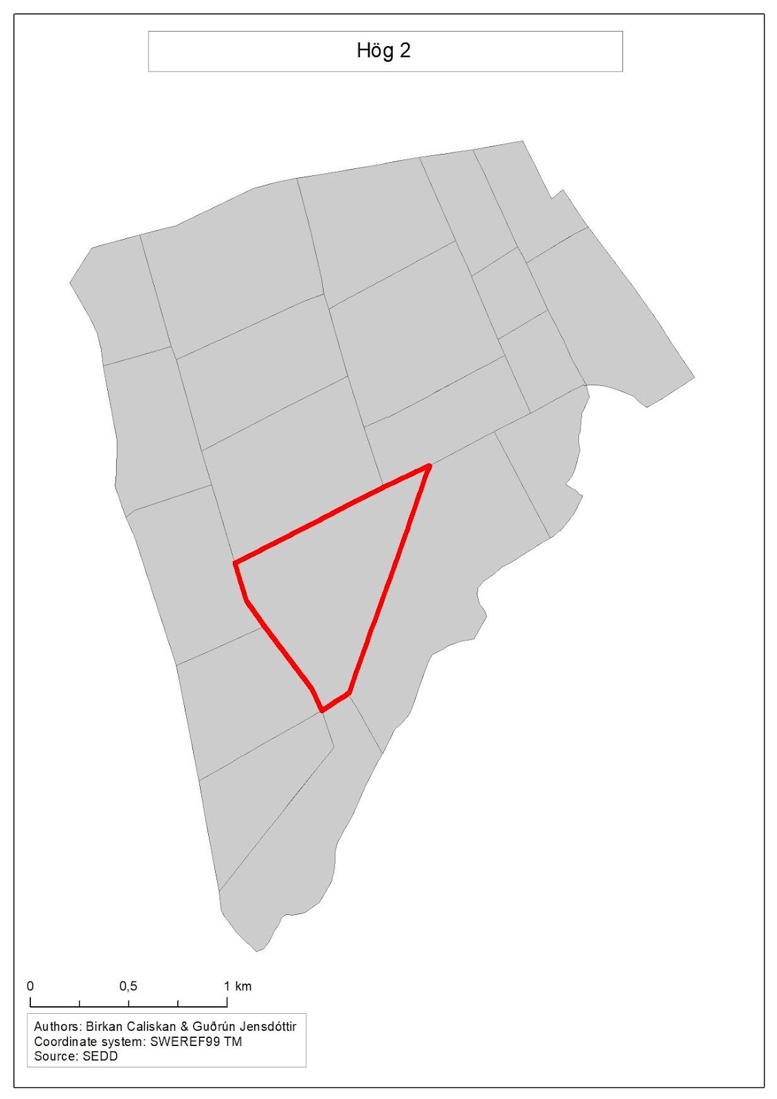
Fig 10. The boundary of Hög 2.
Appendix A - FME flowchart for OSM data
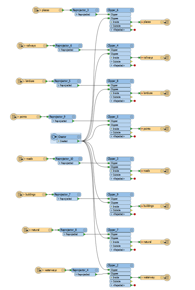
A screenshot from FME software representing the operations performed for OSM dataset.